Week 16 - Dual Use Technologies - Quantum Computing
November 2024 (2216 Words, 13 Minutes)
Yes I know the LateX formatting is bad. Pull the .md from the repo and drop it into Obsidian IDGAF.
In the last few posts, I’ve been looking at the Past and Present of dual-use technologies, and how the American government has attempted to control cryptography research and LLM access to forward its national security goals. In the case of cryptography, we saw how the Government’s attempts to restrict the export of academic cryptographic research was ultimately unsuccessful. We then talked about the current efforts of the Biden administration to reshape industrial policy to bring cutting-edge chip manufacturing stateside.
This week, lets lay the groundwork a technology that has not yet exited the realm of the theoretical. Quantum computing is a proposed improvement to existing computers that would allow computers to solve problems that would be impossible to tackle with the hardware of today. A classical computer like the one you’re using to read this post at its most primitive level a pile of boxes containing either a $0$ or $1$. There is a machine that can look inside the boxes and either spit out new boxes or modify the contents of existing boxes. Each one of these boxes is a bit and is said to be “binary”, as there are only two possible states for each bit. While all the math that allows computers to work can be abstracted to more than 2 states, like trits or quatrits (or digits!) that have three or four (or ten!) possible states respectively, binary systems have become dominant as their relative simplicity plays well with the messy real world where the values of each box isn’t determined by what’s written on a slip of paper, but are instead the voltage of a copper trace on a microchip. Using a ten-based counting system would mean the computers components must successfully discriminate between ten bands of voltage. In a binary system, the electronic components only have to check if a wire is a high or low voltage.

We can combine these boxes to represent more than just $0$ or $1$ by essentially stacking these boxes next to each other. With one box, we’d only be able to represent $0$ or $1$. With two boxes, we can represent four different numbers, being $00$, $01$, $10$, and $11$. Each box essentially represents a place value in a base-2 counting system. In our base-10 counting system, we can represent 1,000 different numbers with up to 3 digits, as $10^3 = 1000$, the $3$ coming from the number digits and the $10$ coming from how many states each digit can represent. By converting this to a base-2 system by swapping the $10$ for a $2$, we’re able to see that we can represent 8 numbers with 3 bits: $2^3 = 8$. This exponential relationship can be abstracted to $2^n = V$ where $n$ is the number of bits and $V$ is the number of values that can be represented. Modern computers can do math on integers that use up to 64 bits, which is about 18 gazillion possible numbers. Using some clever tricks we can also represent decimals, called floating point numbers.
Now that we can represent any number, we need to do something with them. The aforementioned theoretical machine that compares the contents of the boxes and does operations based on their values is a bastardization of the Turing Machine, a thought experiment purported by famed mathematician (and queer icon) Alan Turing.
As it turns out, it’s possible to do all the things a modern computer can do by combining only two primitive logic gates: $AND$ and $NOT$. An $AND$ gate takes two inputs and has one output. It only outputs a $1$ if and only if both input 1 AND input 2 are $1$. A $NOT$ gate takes a single output and inverts it. That means it outputs $0$ if and only if the input is $1$ and outputs $1$ if and only if the input is $0$.
We can plot this out in a helpful “truth table”. For an $AND$ gate, lets call input 1 $i_1$, input 2 $i_2$, and the output $o$:
| $i_1$ | $i_2$ | $o$ | | :—- | :—- | :– | | $0$ | $0$ | $0$ | | $1$ | $0$ | $0$ | | $0$ | $1$ | $0$ | | $1$ | $1$ | $1$ | And for $NOT$:
| $i$ | $o$ | | :– | :– | | $0$ | $1$ | | $1$ | $0$ | These gates can be cleverly combined in a whole bunch of different ways to create build a Turing complete machine! This is pretty fortunate, as we’ve been able to build $AND$s and $NOT$s to be incredibly small, cheap to manufacture, and to have above above-NASA levels of reliability using modern transistors.
The issue with classical bits is that each bit can only represent a single state. Take a theoretical math function $f$ that takes in eight $0$’s or $1$’s (or a byte of information) and spits out a number between 0 and 1. This would be written as $f({0\ 1}^8)$, with ${0\ 1}^8$ being any combination of $0$ and $1$ Your goal is to find an input that returns exactly $0.7326$, or mathematically find ${0\ 1}^8$ where $f({0\ 1}^8) = 0.7326$. It’s pretty simple to intuit that there are only $2^8$ possible inputs for $f$, so you only need to check $2^8$ or $256$ possible inputs in the worst-case scenario to get the desired input. $256$ is a pretty small number, so you could almost check that many cases by hand, and would be trivial to do with a simple “for” loop in a any programming language.
However, this starts getting really difficult when dealing with extremely complex problems with gazillions of possible answers, like figuring out the properties of a theoretical protein computationally without deriving them experimentally. This has ground breaking applications in drug discovery and biotech. To simulate a theoretical protein with 1000 amino acids, let’s say you need to calculate 100 different characteristics for each amino acid. This can include attributes like bond length, bond angles, polarity, and electronegativity of each molecule. That means you may need to simulate $100^{1000}$ or $10^{2000}$ possible combinations of attributes to come up with the final shape of a protein. If we can run through 100 combinations a second, or say we through a modern data center with the latest hardware and algorithms, perhaps we can churn out 10 million combinations a second, we would be exhaust all possible combinations in $10^{1993}$ seconds, something like $10^{1886}$ times longer than the estimated heat death of the universe. That’s not exactly feasible.
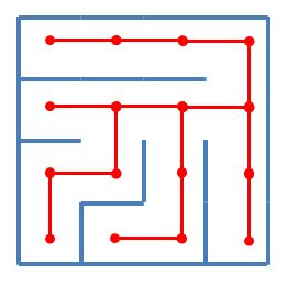
Enter quantum computing. Let’s black-box what the hardware of a quantum computer looks like for this post, and live in the world of mathematics. A way to get around the computational limitation of these problems is to somehow evaluate multiple states at the same time. A good analogy for comparing the difference between classical and quantum algorithms is the problem of solving a maze. This kind of problem can be abstracted into a graph, a favorite data structure of mathematicians and people who actually enjoyed their algorithms class. Each intersection in the maze can be represented as a node in the graph, with potential paths from that node branching off. In a classical implementation, the program might do a depth-first search on the graph, where it traverses as far down in the tree as it can.
The maze solving problem has a linear time complexity, meaning that this will take as many iterations as there are nodes in the graph to find the solution, at least in the worst-case scenario. This is represented with big-O notation: $O(n)$. This means that it would take at most $n$ runs of the algorithm to find the best solution. We call this kind of situation “Linear Time” For the rest of this conversation, remember that the biggest advantage of quantum computers is that they can make that $O$ smaller.
In algorithm analysis, there is a hierarchy of complexity. In the vast majority of cases, especially when the data input size grows, it is much better to run an algorithm that gets the job done in $n$ (linear) iterations than $n^2$ (exponential) iterations. Likewise it is much better to run an algorithm in $\log n$ iterations than one that runs in $n \log n$. The holy grail of course is to run an algorithm in constant time $O(1)$, which takes the same amount of time, regardless of how large the input is. Reducing the computational complexity of certain problems, even going from $O(n^2)$ to $O(n)$, brings them into the realm of the possibility.
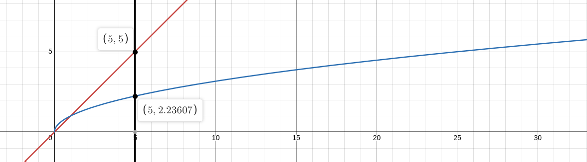
In a theoretical quantum computer, the maze solving problem can be accomplished in $O(\sqrt{n})$ complexity, a “quadratic speedup”. Intuitively, this is a very fast speedup that’s worth pursuing, but the scale of how much faster it is compared to the classical implementation is hard to convey without seeing visually. At five elements, it would take at most 3 ($\sqrt{5} = 2.23$ rounded up $= 3$) iterations of the algorithm before solving the maze.
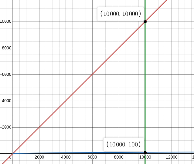
When we zoom out to ten thousand elements, the utility of the speedup is obvious. It would only take a hundred iterations of a quantum depth-first-search algorithm to crawl an entire tree with ten thousand elements!
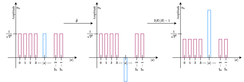
This is due to a phenomenon called quantum annealing. In a classical implementation of a maze-solving Depth First Search algorithm, you only know whether or not you’ve solved the maze. There’s no way for you to “know” how far off you are from finding an optimal solution. Theoretically, each set of conditions you try is just as likely as the next to be the most optimal solution, meaning that the best course of action is to effectively bruteforce the path until you find a solution that works. In a quantum computer, with each iteration you run an algorithm, the “amplitude” or likelihood that your current solution is the optimal one increases and the “amplitude” that other solutions are the solution decreases.
This image shows a single iteration of a quantum algorithm. Notice that the blue “solution” bar increases in height while the red incorrect bars decrease. Think of it as the blue “correct” solution stealing probability from the red “incorrect” solution. Run enough iterations and you can be almost 100% certain that that blue bar is the most optimal solution.
According to the math, a quantum computer can solve any kind of problem that a classical computer can solve, but not necessarily better. The primary learning material I used for this article, quantum.country, gives the example of searching an ordered list for a value. On a classical computer, we use the “Binary Search” algorithm. This algorithm takes an ordered list, evaluates if the midpoint is higher or lower than the target value, and reruns the algorithm on either the top or bottom half of the list until it finds the target value. This has plenty of applications like database searches, an operation that is done trillions of times a second across the world.
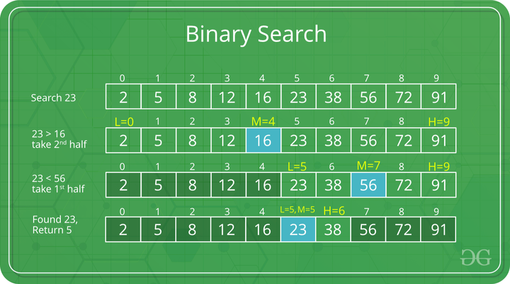
This classical search algorithm has $O(\log n)$ complexity, meaning that for every element that in the list, it takes $\log n$ number of iterations to exhaust the search space.
As we’ll see, quantum computers are not meant to replace classical computers, but instead supplement to help with some very specific problems. That’s not to say that it is impossible for quantum computers to replace classical computers, but instead impractical. Remember what I said about AND’s and NOT gates being the building blocks for all the logic used in a classical computer? We can create those gates in a quantum circuit, which means with enough gates we could fully replicate a computer, with memory, an OS, keyboard inputs etc. In fact, here’s what an AND gate looks like. The inputs on the left are the states of individual qubits. $a$ and $b$ are qubits that are being used in the computation.
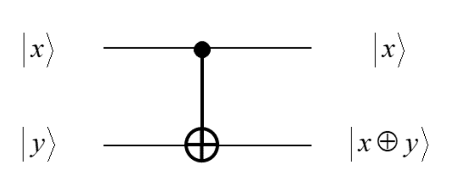 And here’s a Conditional NOT.
Replacing all classical hardware with quantum hardware does not utilize the technology’s strengths. Let’s examine the Quantum Search Algorithm to exemplify this:
The Quantum Search Algorithm
The Quantum Search Algorithm™ is a search algorithm that plays to a quantum computer’s strengths, reducing the complexity of any search to $O(\sqrt n$). This algorithm works by creating a quantum circuit that can evaluate a solution, which provides a solution vector $\ket{s}$, a starting point $\ket{\psi}$, and a fixed point $\ket{E}$. All of these are “vectors”, or linear combinations of quantum states. We can create a “solver” circuit that evaluates to true when a certain condition is met. We can then run the starting state $\ket{\psi}$ through the solver circuit, then reflect about the fixed point vector $\ket{E}$. The resulting vector $\ket{\psi’}$ is going to be WAY closer to the solution $\ket{s}$. It’s a little difficult to understand, so quantum.country provided this super sick graphic:
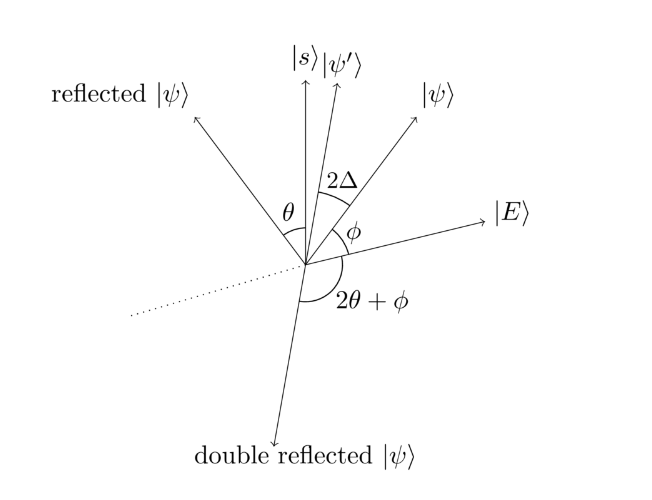
Our goal is to move $\ket{\psi}$ as near as possible to $\ket{s}$. By doing these clever reflections, we can guarantee that $\ket{\psi’}$ is significantly closer to $\ket{s}$ than $\ket{\psi}$ was. The math is really cool, so I absolutely recommend that you go through quantum.country. I’ve done a lot of learning with a lot of different mediums and subjects, and their combination of Anki-style flashcards embedded directly into the content backed by the expertise to explain complex concepts simply is a pedagogical masterpiece.
While a useful quantum computer does not yet exist, researchers have been laying the theoretical framework for creating these machines for about three decades. Next time we talk about quantum computing, we’ll discuss how a future quantum computing industry could used as a tool of power by the US Government.
Music I listened to this week 2 months
Du Hast - Rammstein
Kashmir - Remastered - Reload
ستو أنا - أكرام حسني
St. James Infirmary - The Bridge City Sinners